R for reproducible scientific analysis

Split-apply-combine

Previously we looked at how you can use functions to simplify your code. For example we could define a calcAverageHealth function, which takes the healthData dataset, and calculates the average health metric in the data. We can also define an additional argument so we can filter by HIGroup:

# Takes a dataset and calculates the average health metric for a
# specified study group.
calcAverageHealth <- function(dat, group = "Group 1") {
  healthAverage <- mean(dat[dat$HIGroup == group, ]$health)
  return(healthAverage)
}

A common task you’ll encounter when working with data is that you’ll want to run calculations on different groups within the data. In the above, we are simply calculating the mean health metric in the data. But what if we wanted to calculated the mean health per group, or per education level?

We could, for example, run calcAverageHealth and on each subsetted dataset:

calcAverageHealth(healthData[healthData$education == 4,],"Group 2")

[1] 9.246495

calcAverageHealth(healthData[healthData$education == 5,],"Group 2")

[1] 9.801333

calcAverageHealth(healthData[healthData$education == 6,],"Group 2")

[1] 9.162941

But this isn’t very nice. Yes, by using a function, you have reduced a substantial amount of repetition. That is nice. But there is still repetition. Repeating yourself will cost you time, both now and later, and potentially introduce some nasty bugs.

We could write a new function that is potentially more flexible than calcAverageHealth, but this also takes a substantial amount of effort and testing to get right.

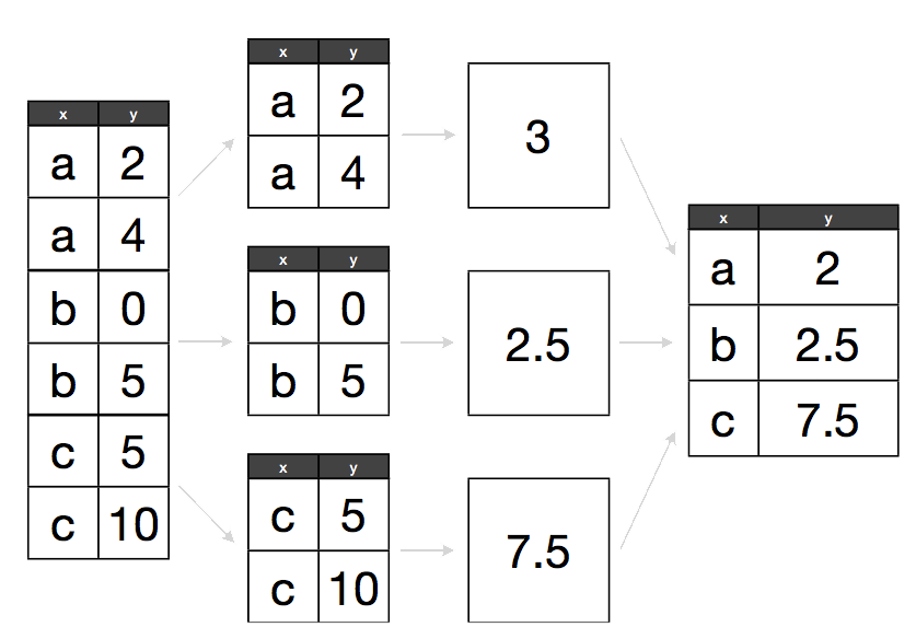
The abstract problem we’re encountering here is known as “split-apply-combine”:

Split apply combine

We want to split our data into groups, in this case education levels, apply some calculations on that group, then optionally combine the results together afterwards.

The plyr package

For those of you who have used R before, you might be familiar with the apply family of functions. While R’s built in functions do work, we’re going to introduce you to another method for solving the “split-apply-combine” problem. The plyr package provides a set of functions that we find more user friendly for solving this problem.

Let’s load plyr now:

library(plyr)

Plyr has functions for operating on lists, data.frames and arrays (matrices, or n-dimensional vectors). Each function performs:

1. A splitting operation
2. Apply a function on each split in turn.
3. Recombine output data as a single data object.

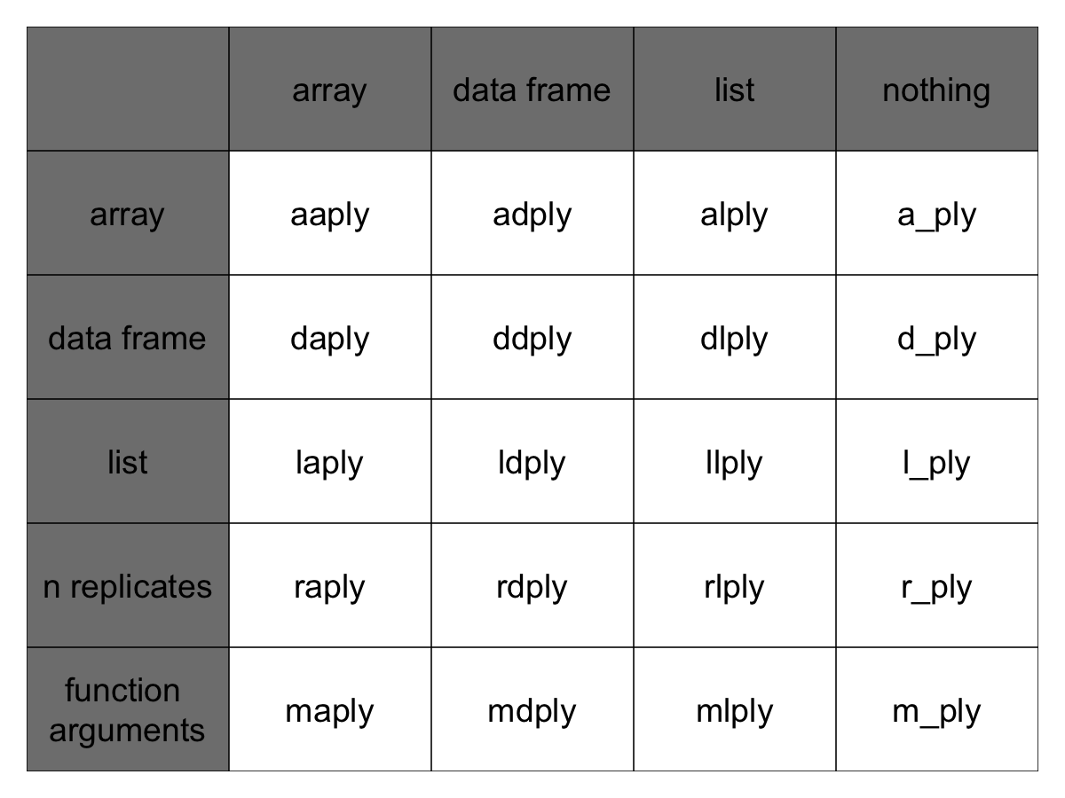
The functions are named based on the data structure they expect as input, and the data structure you want returned as output: [a]rray, [l]ist, or [d]ata.frame. The first letter corresponds to the input data structure, the second letter to the output data structure, and then the rest of the function is named “ply”.

This gives us 9 core functions **ply. There are an additional three functions which will only perform the split and apply steps, and not any combine step. They’re named by their input data type and represent null output by a _ (see table)

Note here that plyr’s use of “array” is different to R’s, an array in ply can include a vector or matrix.

Full apply suite

Each of the xxply functions (daply, ddply, llply, laply, …) has the same structure and has 4 key features and structure:

xxply(.data, .variables, .fun)

• The first letter of the function name gives the input type and the second gives the output type.
• .data - gives the data object to be processed
• .variables - identifies the splitting variables
• .fun - gives the function to be called on each piece

Now we can quickly calculate the mean birth year per education level:

ddply(
 .data = healthData,
 .variables = "education",
 .fun = function(x) mean(x$health)
)

  education       V1
1         1 6.487500
2         2 9.967500
3         3 8.620682
4         4 9.340258
5         5 9.069877
6         6 8.976614
7         7 9.321495
8         8 9.525871
9         9 9.653661

Let’s walk through what just happened:

• The ddply function feeds in a data.frame (function starts with d) and returns another data.frame (2nd letter is a d) i
• the first argument we gave was the data.frame we wanted to operate on: in this case the healthData dataset.
• The second argument indicated our split criteria: in this case the “education” column. Note that we just gave the name of the column, not the actual column itself like we’ve done previously with subsetting. Plyr takes care of these implementation details for you.
• The third argument is the function we want to apply to each grouping of the data. We had to define our own short function here: each subset of the data gets stored in x, the first argument of our function. This is an anonymous function: we haven’t defined it elsewhere, and it has no name. It only exists in the scope of our call to ddply.

What if we want a different type of output data structure?:

dlply(
 .data = healthData,
 .variables = "education",
 .fun = function(x) mean(x$health)
)

$`1`
[1] 6.4875

$`2`
[1] 9.9675

$`3`
[1] 8.620682

$`4`
[1] 9.340258

$`5`
[1] 9.069877

$`6`
[1] 8.976614

$`7`
[1] 9.321495

$`8`
[1] 9.525871

$`9`
[1] 9.653661

attr(,"split_type")
[1] "data.frame"
attr(,"split_labels")
  education
1         1
2         2
3         3
4         4
5         5
6         6
7         7
8         8
9         9

We called the same function again, but changed the second letter to an l, so the output was returned as a list.

We can specify multiple columns to group by:

ddply(
 .data = healthData,
 .variables = c("education","sex"),
 .fun = function(x) mean(x$health)
)

   education    sex        V1
1          1 Female  4.145000
2          1   Male  8.830000
3          2 Female  9.885000
4          2   Male 10.050000
5          3 Female  7.688125
6          3   Male  9.153571
7          4 Female  9.158053
8          4   Male  9.470570
9          5 Female  8.764062
10         5   Male  9.269592
11         6 Female  8.760938
12         6   Male  9.195714
13         7 Female  9.059946
14         7   Male  9.562327
15         8 Female  9.517341
16         8   Male  9.535098
17         9 Female  9.469059
18         9   Male  9.755552

daply(
 .data = healthData,
 .variables = c("education","sex"),
 .fun = function(x) mean(x$health)
)

         sex
education   Female      Male
        1 4.145000  8.830000
        2 9.885000 10.050000
        3 7.688125  9.153571
        4 9.158053  9.470570
        5 8.764062  9.269592
        6 8.760938  9.195714
        7 9.059946  9.562327
        8 9.517341  9.535098
        9 9.469059  9.755552

You can use these functions in place of for loops (and its usually faster to do so): just write the body of the for loop in the anonymous function:

d_ply(
  .data=healthData,
  .variables = "education",
  .fun = function(x) {
    meanHealth <- mean(x$health)
    print(paste(
      "The mean health metric for education level", unique(x$education),
      "is", meanHealth
   ))
  }
)

[1] "The mean health metric for education level 1 is 6.4875"
[1] "The mean health metric for education level 2 is 9.9675"
[1] "The mean health metric for education level 3 is 8.62068181818182"
[1] "The mean health metric for education level 4 is 9.34025830258303"
[1] "The mean health metric for education level 5 is 9.06987654320988"
[1] "The mean health metric for education level 6 is 8.97661417322835"
[1] "The mean health metric for education level 7 is 9.32149484536082"
[1] "The mean health metric for education level 8 is 9.52587127158556"
[1] "The mean health metric for education level 9 is 9.65366108786611"

ddply(
  .data = healthData,
  .variables = healthData$education,
  .fun = function(dataGroup) {
     mean(dataGroup$conscientiousness)
  }
)

ddply(
  .data = healthData,
  .variables = "education",
  .fun = mean(dataGroup$conscientiousness)
)

ddply(
  .data = healthData,
  .variables = "education",
  .fun = function(dataGroup) {
     mean(dataGroup$concientiousness)
  }
)

adply(
  .data = healthData,
  .variables = "education",
  .fun = function(dataGroup) {
     mean(dataGroup$conscientiousness)
  }
)